Geographical-Data-Analysis-of-Poverty-in-Italy-with-R

Geographical Data Analysis of Poverty in Italy

This project explores poverty in Italy through a geographical and statistical perspective, using data from ISTAT and BES (Benessere Equo e Sostenibile).
The analysis combines descriptive statistics, spatial autocorrelation tests, and spatial regression models to highlight territorial inequalities and socio-economic drivers of poverty.

The analysis is based on a poverty rate dataset from Italian Statistical Institute ISTAT avaiable here that contains 8 sociodemographic variables listed here and is analized by 5 main scripts in src descripted here

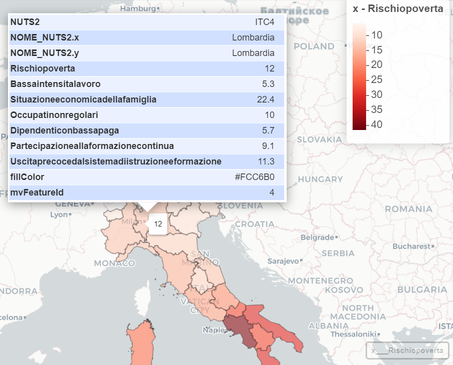
• Interactive map of poverty risk in Italy
• ↓ Screenshot from the Interactive map ↓

• 

Objectives

• Analyze the risk of poverty across Italian regions
• Study socio-economic differences using BES indicators
• Apply spatial autocorrelation tests (Moran’s I, Geary’s C)
• Compare spatial regression models (SAR, SAC)

---

Workflow

1. 01_data_preparation.R → Load shapefile and poverty dataset, merge, clean, and explore.
2. 02_exploratory_analysis.R → Descriptive statistics, plots, and OLS baseline models.
3. 03_spatial_weights.R → Build spatial weight matrices (Queen contiguity).
4. 04_spatial_tests.R → Moran’s I, Geary’s C, and Local Indicators of Spatial Autocorrelation (LISA).
5. 05_spatial_models.R → Estimate SAR and SAC spatial regression models, compare AIC, compute direct and indirect effects.

---

Technologies

• Language: R
• Main Libraries:
  • sf – spatial data handling
  • spdep – spatial dependence models
  • ggplot2 – data visualization
  • dplyr – data wrangling

---

Key Results

Regression Analysis

The linear regression model identifies the main drivers of poverty risk:

• Low work intensity: strong positive and highly significant effect. Regions with lower labor intensity show higher poverty risk.
• Household economic situation: negative and significant. Better family economic conditions reduce poverty risk.
• Continuous training participation: negative and significant. Lifelong learning acts as a protective factor against poverty.
• Early school leaving: positive and significant. Dropping out of education increases poverty risk.

The model shows excellent fit (Adjusted R² = 0.98), confirming that these socio-economic variables explain most of the variance in poverty risk.

---

Spatial Effects (SAC Model)

The spatial autoregressive model highlights that poverty is not randomly distributed, but spreads across neighboring regions:

• Low work intensity: strong positive direct effect, but negative indirect effect on neighboring areas (suggesting compensatory dynamics).
• Household economic situation: positive indirect effect, meaning economic hardship in one region tends to spill over into adjacent areas.

These findings imply the need for coordinated regional policies, since poverty dynamics do not stop at administrative borders.

---

Spatial Autocorrelation (Moran’s I and Local Moran)

• 
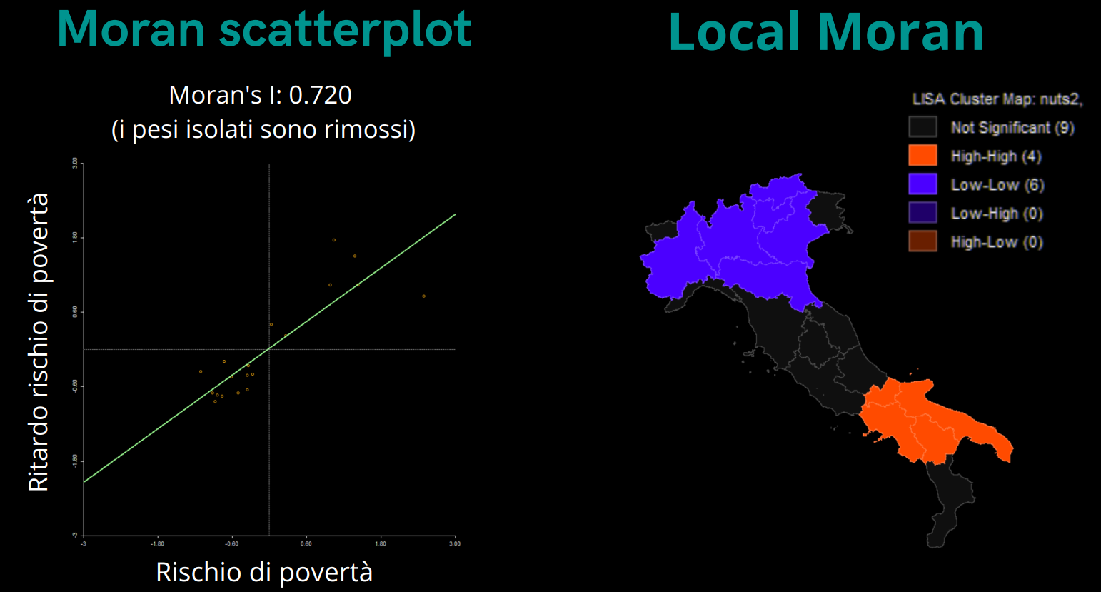
• Moran’s I = 0.72 → strong positive spatial autocorrelation. High-poverty regions cluster together, as do low-poverty regions.
• LISA Cluster Map:
  • High-High cluster: Southern Italy (critical poverty risk hotspot).
  • Low-Low cluster: Northern Italy (low poverty risk concentration).
  • No regions fall into Low-High or High-Low outliers.

---

Conclusions

• Poverty risk in Italy is strongly linked to labor conditions, household economy, and education.
• The phenomenon has a clear spatial dimension, with persistent North-South disparities.
• 
• Policy implications:
  • Invest in quality employment and lifelong learning.
  • Develop interregional strategies, since poverty spreads across territories.
• Poverty in Italy is not only a social issue, but also a spatial one:
  it concentrates in specific areas and propagates across neighboring regions, calling for comprehensive and territorial policies.

---

References

• ISTAT – Italian National Institute of Statistics
• BES Project – Equitable and Sustainable Well-being indicators
• European Pillar of Social Rights (EPSR)
• Italian National Recovery and Resilience Plan(PNRR)

## From a F.Cecere, G.Masiello & S.Spagnuolo collaboration.

This site is open source. Improve this page.